DRIFT-SCAN TIMING OF
ASTEROID OCCULTATIONS
John Broughton
(Updated 2014-11-13)
 Occultations present the opportunity to remotely
investigate shape and dimensions of planetary objects with orders of
magnitude gain in resolution over direct imaging. I have in the past
observed visually a spectacular Jupiter occultation of 2.6-magnitude
Beta SCO and measured brief disappearances of a fifth magnitude star
by ringlets of Saturn but until 2003 I had never observed the more
common variety of occultation by an asteroid. Following on from
the development of Dave Herald’s Occult
software, the turning point came with the advent of Steve Preston’s
updated
predictions, the accuracy of which made viable a CCD imaging and
timing technique I had under consideration many years earlier. The
original inspiration was a trailed photograph of a Metis occultation
taken by Paul Maley in 1979.
Occultations present the opportunity to remotely
investigate shape and dimensions of planetary objects with orders of
magnitude gain in resolution over direct imaging. I have in the past
observed visually a spectacular Jupiter occultation of 2.6-magnitude
Beta SCO and measured brief disappearances of a fifth magnitude star
by ringlets of Saturn but until 2003 I had never observed the more
common variety of occultation by an asteroid. Following on from
the development of Dave Herald’s Occult
software, the turning point came with the advent of Steve Preston’s
updated
predictions, the accuracy of which made viable a CCD imaging and
timing technique I had under consideration many years earlier. The
original inspiration was a trailed photograph of a Metis occultation
taken by Paul Maley in 1979.
CCD
Due to their slow image transfer rate,
most astronomical CCD cameras cannot record short-term variability on
consecutive frames without missing out on most of the action; hence
an occultation is best recorded on a single frame. One technique that
has been particularly useful in recording rapid changes during lunar
occultations is called TDI (time delay integration) where the CCD
array is read out line by line to produce a trailed image. Not many
cameras including my own have operating software supporting this
electronic option but any integrating camera attached to a stationary
telescope can take trailed images as a consequence of Earth’s
extremely regular rotation, which just happens to provide a rate of
motion well suited to recording asteroid occultations.
With the advantage of noise reduction, a cooled CCD
camera provides a substantial magnitude gain over non-integrating
video cameras. From a moderately light-polluted location under
otherwise favourable circumstances, sidereal-rate star trails as
faint as magnitude 14 can be acquired with a telescope of 25cm
aperture. A single image provides a convenient record for analysis,
producing in most cases an unambiguously positive or negative result.
Although cloud induced disappearances can mar an observation, they
equally affect all nearby trails, making them easy to differentiate
from the real thing.
Rigorous timing methods were devised and first
employed for the Lutetia occultation of August 24, 2003. An accuracy
of around .05 second can be expected for well-recorded events,
leading to kilometre resolution in chord length and potentially an
extremely precise celestial position for the asteroid. Lutetia
incidentally has since been announced by ESA as the major asteroid
flyby target of its currently enroute Rosetta comet rendezvous
mission. Events previously considered unobservable may be within
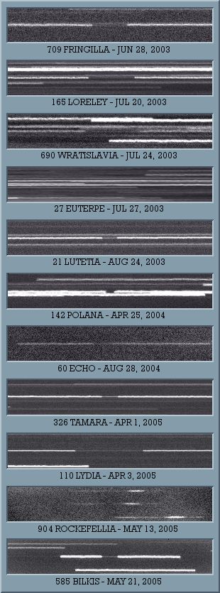
reach of observation; at right are the first 11 positive occultations
recorded from my Reedy Creek, Gold Coast observatory in eastern
Australia. The Euterpe event had a 0.3-magnitude drop, Echo occulted
a star of magnitude 11.9 only 15 degrees from a full moon and the
Rockefellia occultation was observed through cloud! Over a
six-year period, 45 positive asteroid and dwarf-planet occultations
have been recorded from the one location, all but four being
drift-scan observations. Drift-scan reports appear from time to
time on RASNZ’s Occultation Section results
pages and also on the site are commented predictions
for Australasia.
COORDINATING CCD AND VIDEO DRIFT-THROUGH OBSERVATIONS
The
telescope is pre-pointed to a fixed position in the sky where by
virtue of Earth’s rotation; the target will drift through the
centre of field at the time of occultation. Because the trail ends of
drift scans are used in the timing calculations, the exposure must
begin and end while the star is within the frame boundary, therefore
it is important to employ accurate and fail-safe methods of
coordinating both telescope and camera, especially when the field of
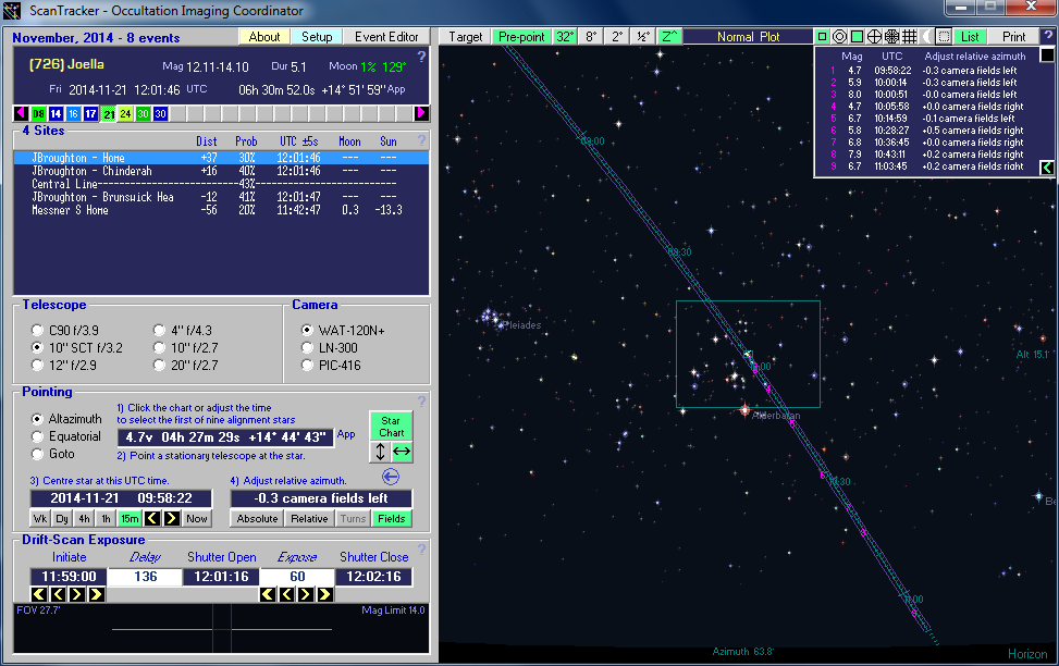
view is small. Originally developed in 2004, ScanTracker now includes
three pre-pointing modes and a printable chart of alignment stars,
making it easy to point all kinds of telescopes whether used for
drift scan, video or visual drift-through observations. The new modes
enable an alignment on a naked-eye star followed by a single-axis
offset and no faint-star hopping is required. Altazimuth mode is
especially useful for rapid set up of portable telescopes. Recent
developments include an extension of the charted limiting magnitude
from 6 to 12; dispensing with the need to rely on other planetarium
software for alignments in any mode. Version 5 released in September,
2014 is freely available here.
View the readme file for instructions.
The camera is preferably oriented north up to produce
left to right drift along rows of the CCD array; quite straight
forward on a polar-aligned equatorial. For an altazimuth SCT, the
east-west line of occultation displayed in ScanTracker will give an
idea of the orientation. Final adjustments can be made with the aid
of trial and error imaging of star trails.
In the drift-scan exposure section, its length
is adjustable from 10 seconds up to a maximum dependant on field
width and declination. An exposure 20 times longer than
duration of the occultation is necessary if you want to cover the
region in which an asteroid satellite could reside. Exceeding this
can be disadvantageous since there is loss of limiting magnitude by
sky glow the longer the exposure lasts. A 200 second exposure for
instance may lose 2 magnitudes over one of 20 seconds at a moderately
light-polluted site. For this reason it is good practise to shorten
the exposure if circumstances are unfavourable for obtaining a well
recorded image such as might be caused by bright moonlight or
twilight, poor seeing, small magnitude drop, low elevation or
combinations thereof. A minimal exposure should always be
employed when there is threat of obscuration by cloud. With
reference to an updated prediction, a rule of thumb I use to find
minimum exposure is to add the maximum duration of the occultation to
the time uncertainty plus 15 seconds for some margin of safety.
Another reason to use an exposure shorter than the maximum allowed
for your field-width is to avoid an overlap by a trail of equivalent
or brighter magnitude. Such overlaps contain their own
contrast-reducing seeing variations. GUIDE
8 with UCAC stars enabled is my preferred planetarium software
when checking a target’s surroundings for interfering stars
lying within 8 arc seconds of the same declination and within the
intended exposure length in seconds of RA. In general, a drift scan
of an occultation fainter than Magnitude 13.5 in a crowded field is
not likely to produce measurable results.
The simulated drift scan at the bottom of ScanTracker
displays the field of view and estimated limiting magnitude relevant
to the selected telescope-camera combination. The magnitude
represents the faintest star whose occultation is potentially
detectable under favourable moonless conditions. A 2-magnitude
loss from the listed limit can be expected when a full moon is
present.
MANUAL TIMING OF THE
EXPOSURE
In the Windows operating system, the time listed in
image file headers can easily be off by a second, even shortly after
setting the clock and as in my case the exposure length may not be
exactly as commanded, so for timing occultations I disregard this
information. Because computer equipment floods short-wave with
static, a digital timer previously synchronised to WWVH can be
visually monitored during the beginning and end of exposure. If the
camera lacks an audible shutter, a cardboard disk taped to a tennis
racket can be used to unblock and block the telescope aperture
(without actually touching the telescope) at the intended times
within an electronic exposure a few seconds longer in duration. If as
is preferable the camera has a mechanical shutter, the times when the
shutter is heard to open and close are written down with the
fractional second part estimated. Either method may be as accurate as
0.2-second, depending on the individual.
RIGOROUS TIMING
OF THE MECHANICAL SHUTTER
A $10 quartz analogue clock
provides a low-cost means to derive accurate timing of the sub-second
part, using the ticking sound. The small unit containing the workings
can be removed from the clock and placed in contact with a
microphone. Audio tests on mine revealed an hourly drift rate of only
.008 second! The battery can be inserted by trial and error
until the ticking is heard synchronized with short-wave UTC. This is
then recorded on one channel of a stereo tape recorder while UTC is
simultaneously recorded on the other through a second microphone or
line-in. This recording is done prior to, or after the event
when computer and camera equipment are not operating and causing
radio interference to the short-wave signal. The microphone that
recorded from the radio is then fastened in contact with the CCD
camera to record its shutter clicks during the occultation. As in the
first recording, the clock ticks are recorded on the other channel,
guaranteeing a clear time signal at the critical time. It’s
possible to make the drift-scan observation autonomous in order to
observe the same event from another site. Both ScanTracker and MaxIm
DL support delayed exposures of up to 32768 seconds (9.1 hours). The
tape recorder could be on a power-point timer and an alarm set up to
go off at the beginning of a specific minute and be audible on the
clock-tick channel.
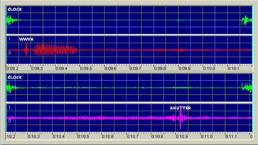 Audio
software such as Audacity
is later used to analyse both stereo recordings in deducing the times
the shutter opened and closed relative to UTC, as is shown in the
diagram of a 1-second interval between clock ticks. Such timing
measurements done within second intervals are not prone to errors
caused by tape stretch. If the short-wave signal is faint and
immersed in static, the clearest part of the recording can be
selected, the volume maximised and noise reduction button pressed a
few times until the UTC second marker stands out more clearly. The
spike in the audio plot repeats every second in the same place
relative to the clock tick. In my experience if the signal can be
heard, then its position can be measured. To correct for propagation,
0.01-second for every 3000 km from the short-wave transmitter should
then be added to the shutter timings.
Audio
software such as Audacity
is later used to analyse both stereo recordings in deducing the times
the shutter opened and closed relative to UTC, as is shown in the
diagram of a 1-second interval between clock ticks. Such timing
measurements done within second intervals are not prone to errors
caused by tape stretch. If the short-wave signal is faint and
immersed in static, the clearest part of the recording can be
selected, the volume maximised and noise reduction button pressed a
few times until the UTC second marker stands out more clearly. The
spike in the audio plot repeats every second in the same place
relative to the clock tick. In my experience if the signal can be
heard, then its position can be measured. To correct for propagation,
0.01-second for every 3000 km from the short-wave transmitter should
then be added to the shutter timings.
GPS
More
conveniently, the short-wave time signal and clock can be replaced by
a GPS-based timer for simultaneous recording with the shutter clicks,
in which case only a single stereo recording is necessary and
propagation does not apply. Suitable devices are the KIWI
beeper system, the GPS
Clock and the VNG-uc
GPS Time Signal Generator. This last one is the only fully
self-contained GPS timing device capable of recreating short-wave UTC
signals but hasn't been put into production.
ELECTRONIC
SHUTTERS
Cameras lacking mechanical shutters give no audible
cue we can use to time the exposure, so a different approach is
required. A tie-clip mike can be attached to the RA drive motor
instead of the camera. If sidereal tracking is turned on for just a
second or two near each end of the exposure, a star image will show
up near each end of the trail to become measurement points instead of
the trail ends themselves. From the audio recording of the time
signal and drive motor noise, it is the time of the end of the first
short tracking period and beginning of the second that represent the
star image centres on the trail. The tracking periods are kept short
to minimise any degradation of timing accuracy by periodic error.
I’ll later refer to trails of this type as having star-bump
profiles to distinguish them from normal ones.
IMAGE ANALYSIS
As
with any CCD image, the drift scan should be calibrated with bias,
dark and flat field frames to achieve the highest signal to noise
ratio. Contrary to popular belief, timing resolution of an
occultation using a CCD drift image is not limited by pixel size,
except in unlikely events of very short duration. Trail ends can be
measured at the sub-pixel scale by interpolation of the values
contained in adjacent pixels; in effect joining the dots to find the
point where the profile crosses a certain brightness level. For best
results, the whole width of the trail needs to be taken into account
by averaging X values over several rows on the Y-axis. In MaxIm
DL this can be achieved automatically using a horizontal box
aperture. First though it may be necessary to precisely level
the trail using the edit menu rotate function with the bicubic
resample box ticked. Next hold down the left mouse button to drag a
long narrow aperture around the trail starting at the left edge of
the frame, excluding any adjacent trails and as much background as
possible. Then use the view menu line profile function, select
horizontal box and the mean sample option and press the export button
to save it to disk in the form of a
comma-separated-values file.
A normal profile is a
stretched version of a fixed star’s bell-shaped curve and being
a time variable image, it is modified by atmospheric turbulence.
Calculations I did in 2004 showed the end of trail profile to be
stretched 200% compared to that of a fixed-star radius, and the point
of origin to be located exactly midway in height between the trail
and background levels. Measurement levels derived from the
lengths of many rigorously timed trails in 2003 averaged within 1% of
the 50% level. Even under the influence of diffraction, the
measurement level of the occulted part was calculated to be at or
very close this level so I believe diffraction to be self-cancelling
in the case of sidereal-rate drift scans. This is different from the
measurement level of high-frame-rate video recordings where
diffraction theory indicates should be made at the 25% level.
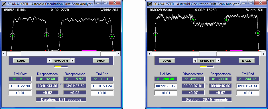
SCANALYZER
This
trail measuring application includes dynamic vertical scaling,
smoothing of scintillation and signal noise, cancellation of optical
distortion effects and calculation of overall timing accuracy. The
LOAD button facilitates loading a profile such as included example
file 050521 Bilkis.csv. The four measurements on the profile
are always made in left to right order. Clicking the plot produces an
expanded view whose width in pixels can be zoomed in as far as 32 or
all the way out using those arrows that appear either side of the
SMOOTH button. Clicking in this expanded view where the levels change
brings about a sub-pixel X measurement displayed in green. A right
click returns the full profile where the next position can be
selected. Once the fourth measurement is made, times for the
occultation based on the 50% level are computed and displayed.
Measurements can be re-done by use of the BACK button.
Scanalyzer recognises and can measure star-bump profiles, in which
case ‘Star Bump’ replaces the terms ‘Trail Start’
and ‘Trail End’ after the first position is measured.
Since in practice the
moving star is a distribution of light on the CCD two or more pixels
wide, sudden changes caused by an occultation always have a slope and
are less abrupt than the rapid variations due to scintillation and
signal noise. The SMOOTH button applies a gaussian filter to suppress
this high-frequency interference and improve accuracy without biasing
the measurements. Smoothing should be applied at least once and can
be done twice in the case of poor seeing conditions. On the third
press, the original raw state is restored. Lights below the button
indicate the level of smoothing and timing results are updated
automatically.
When loading a
CSV profile file, Scanalyzer also loads a TXT file of the same name
if present in the same directory. Previously edited in Notepad by the
user, this file holds two lines for trail-end shutter timing followed
by one line for accuracy, followed by four lines of astrometric data
used in averting a distortion-induced warp in timing. If this
file is absent, timings can be manually entered into the white boxes
or alternately the file can be present but omitting the four lines of
astrometry. Lacking astrometry, computations are based on a simple
extrapolation of image coordinates to time, which scarcely matters in
the case of telescopes with negligible distortion such as unmodified
SCTs. On the other hand a focal reduced SCT will have a little
distortion while Newtonians and Cassegrains suffer considerably more.
The astrometric data can be measured from any image taken with the
same optical configuration. After calibration to celestial
coordinates using Astrometrica,
four positions are measured near the X and Y image coordinates
equivalent to trail start (alternately star-bump), disappearance,
reappearance and trail end (alternately star-bump). A
Ctrl-click operation enables measurement within a pixel or two of
where intended and the X parameter is displayed to two decimal places
in the PSF-Fit box. This figure is to be manually incorporated into a
contiguous object name of the form X468.55 when saving a position. X
can be followed by anything up to 4096 but there must be no spaces.
The four lines of data are then copied from Astrometrica’s
MPCReport.txt and added to the timings as in the example file 050521
Bilkis.txt. These positions show up as red dots in the Scanalyzer
profile plot to indicate astrometric data is loaded and verify their
locations align approximately with the four measurement positions.
Relative scales between these astrometric positions are derived and
applied as corrections to the timings.
Faintly recorded
occultations having depth comparable to the amplitude of seeing
irregularities and random noise might produce what is obviously a bad
measurement. A hump or hollow may interfere where a level is being
averaged or could cause the profile slope to level out temporarily
just where X is being interpolated. In such cases the keyboard
Ctrl-up and Ctrl-down arrow keys enable modification of the profile
at the position of the cursor. This is best done after returning the
profile to an unfiltered and unmeasured state via the SMOOTH and BACK
buttons. After adjustments to the problem area, the profile is
resmoothed and remeasured. Keep in mind that such modifications
disappear if the profile is again restored to its original state.
Timing accuracy
is derived from the sum of the audio recording measurement
uncertainty and profile measurement uncertainties for both
occultation and trail end. The latter calculations involve a
simulated drop in light in an unocculted part of the profile made at
a string of consecutive pixel locations before being averaged. A
magenta coloured line represents that region. The Bilkis drift-scan
observation made with a 0.5-m telescope seems to indicate that for
larger apertures, the best events measured in Scanalyzer will
approach 0.01-second accuracy once the audio measurement uncertainty
is effectively zeroed with the aid of direct GPS-based timings.
Scanalyzer is free to download here.
ACKNOWLEDGEMENTS
The camera used by the author was
acquired following a Planetary Society Gene Shoemaker NEO research
grant. Keith Gelling made diffraction calculations on an example
asteroid occultation. I thank the principal members of IOTA and the
RASNZ Occultation Section for recognizing the value of this work.
CONTACT
jbroughton2(at)dodo(dot)com(dot)au
LINKS IOTA
Euraster
RASNZ
Occult
Updated
Predictions Guide
8 MaxIm DL
Astrometrica
Audacity
ScanTracker
Scanalyzer